
Fake News Classification with Tensorflow
In this blog post, we will be developing a text classifier using TensorFlow that can detect misinformative news articles. We will be using a dataset from kaggle containing the titles and complete text from labeled ‘fake’ and ‘not fake’ news articles.
Step 1: Acquire our training data from the dataset.
Our test and training data have already been seperated and stored into urls, feel free to copy this snippet to load the data:
train_url = "https://github.com/PhilChodrow/PIC16b/blob/master/datasets/fake_news_train.csv?raw=true"
Next, we will import the relevant packages:
import tensorflow as tf
import numpy as np
import pandas as pd
Let’s read in the dataset and inspect our data.
train_df = pd.read_csv(train_url)
print(train_df.shape)
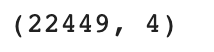
train_df.head()
 Notice that the ‘'’title’’’ column contains the title of each article, and the “text” column contains the complete text. Finally, the “fake” column specifies whether the article is fake or not, where 0 corresponds to real and 1 corresponds to fake.
Step 2: Make the dataset for text classification
First, we will remove the stopwords:
import nltk
#import stopwords from nltk
nltk.download('stopwords')
Next, we will write a function to make a tf.data.Dataset from our data which will remove stopwords from the titles and text, and thus will have two inputs (title and text), and one output (the classification; i.e. whether the article is classified as fake or not.)
def make_dataset(df):
#remove stopwords from text and title
stop = stopwords.words('english')

df['title'] = df['title'].str.lower() #first change to lowercase
df['text'] = df['text'].str.lower()

df['title'] = df['title'].apply(lambda x: ' '.join([word for word in x.split() if word not in (stop)]))
df['text'] = df['text'].apply(lambda x: ' '.join([word for word in x.split() if word not in (stop)]))

#make dataset
my_data = tf.data.Dataset.from_tensor_slices(
  ({"title" : df[["title"]], "text" : df[["text"]]}, {"fake" : df[["fake"]]}) #two inputs, and one output
)
my_data = my_data.batch(100)
return my_data
Make Training/Validation Data
We can now make our dataset using this function:
data = make_dataset(train_df)

data = data.shuffle(buffer_size = len(data)) #shuffle the data
# 80% train, 20% validation
train_size = int(0.8*len(data))

train = data.take(train_size)
val   = data.skip(train_size)
After running this, we get a batch size of 180 for our train data and 45 for our validation data, since we do an 80% vs. 20% split.
Calculate Base Rate
Let’s calculate the base rate, i.e. the rate of accuracy for guessing the most likely outcome.
print(train_df.shape[0])
print(train_df['fake'].sum())
base_rate = train_df['fake'].sum() / train_df.shape[0]
print(base_rate)
 As we can see, guessing ‘fake’ every time would give our model an accuracy of approximately 52.3%
Text Vectorization
In this model, we will also be using a text vectorization layer that we will prepare here:
from tensorflow.keras.layers.experimental.preprocessing import TextVectorization
import re
import string

#preparing a text vectorization layer for tf model
size_vocabulary = 2000

def standardization(input_data): #turn text into lowercase and remove punctuation
    lowercase = tf.strings.lower(input_data)
    no_punctuation = tf.strings.regex_replace(lowercase,
                                  '[%s]' % re.escape(string.punctuation),'')
    return no_punctuation

title_vectorize_layer = TextVectorization( #vectorize the text
    standardize=standardization,
    max_tokens=size_vocabulary, # only consider this many words
    output_mode='int',
    output_sequence_length=500)

title_vectorize_layer.adapt(train.map(lambda x, y: x["title"]))
In these last lines, we preemptively call the text vectorization on our titles, preparing the layer for our first text classification model…
Step 3: Creating our Models!
We will be creating multiple text classification models to determine the answer to the following question:
When detecting fake news, is it most effective to focus on only the title of the article, the full text of the article, or both?
In order to answer this question, we can construct three models, one using only the titles, one using only the text, and finally, a model using both the titles and text.
First let’s import relevant packages:
from tensorflow import keras
from tensorflow.keras import layers
from tensorflow.keras import losses
Now we can implement our models using keras.
Let’s start with the titles. We will be using the Functional API.
title_input = keras.Input(shape = (1,), name = 'title', dtype = 'string') #input layer
title_x = title_vectorize_layer(title_input)
title_x = layers.Embedding(size_vocabulary, 10, name = "title_embedding")(title_x) #10 dimension embedding layer
title_x = layers.Dropout(0.2)(title_x) #drop 20% of data
title_x = layers.GlobalAveragePooling1D()(title_x)
title_x = layers.Dropout(0.2)(title_x)
title_x = layers.Dense(32, activation='relu')(title_x)
title_output = layers.Dense(2, name = 'fake')(title_x) #2 classes, either fake or not fake
model1 = keras.Model(inputs = title_input, outputs = title_output)
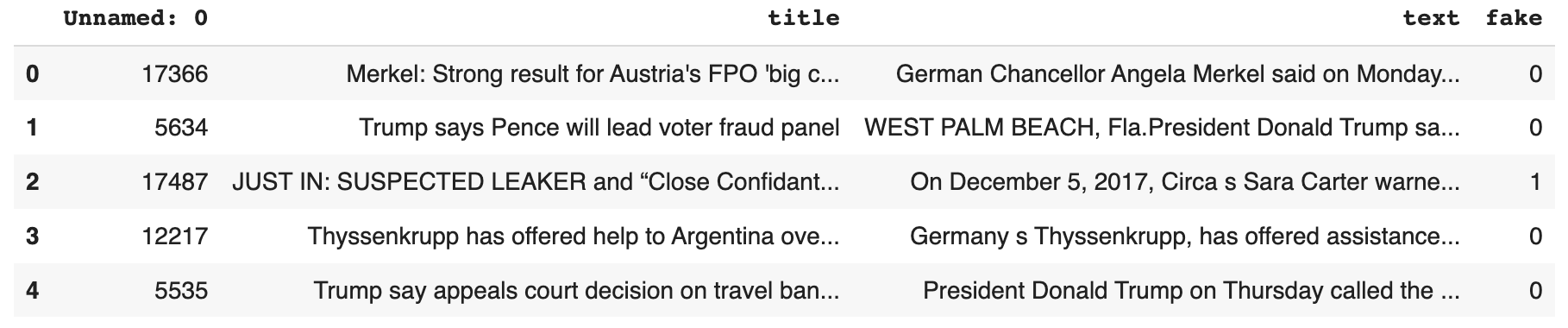
model1.summary()
 Notice, we specify the shape of our input using the keras.Input() function, and we utilize our vectorized titles, an embedding layer, some dropout layers, a pooling layer, and finally two dense layers.
Now we can compile and fit our model with the following code:
model1.compile(optimizer = "adam", #compile the model
loss = losses.SparseCategoricalCrossentropy(from_logits=True),
metrics=['accuracy']
)
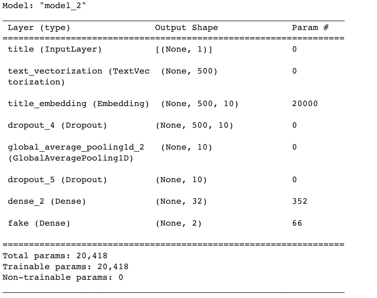
history = model1.fit(train, #train the model
validation_data=val,
epochs = 10,
verbose = True)
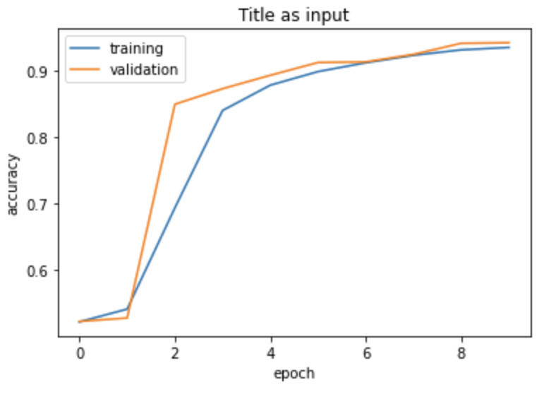
 As you can see, at epoch 10, we get a relatively strong validation accuracy of 94.22%, however your training performance may have been slightly different.
Let’s visualize the performace of our model.
from matplotlib import pyplot as plt
#define model performace history plotting function
def plot_history(history, title = "type of input"):
  plt.plot(history.history["accuracy"], label = "training")
  plt.plot(history.history["val_accuracy"], label = "validation")
  plt.gca().set(xlabel = "epoch", ylabel = "accuracy")
  plt.title(f"{title} as input")
  plt.legend()

plot_history(history, title = "Title")
Next, lets train a model on only the text of the news articles.
Just as before, we vectorize our text and create the model with the same exact specifications, which will be useful for model comparison.
vectorize_text = TextVectorization( #same as title model
standardize=standardization,
max_tokens=size_vocabulary,
output_mode='int',
output_sequence_length=500) #length 500
vectorize_text.adapt(train.map(lambda x, y: x["text"]))
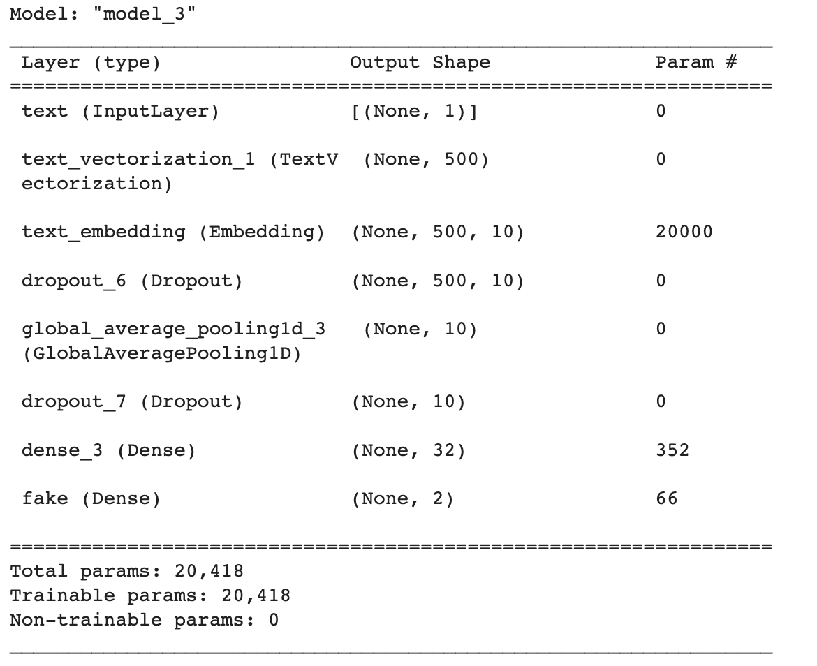
text_input = keras.Input(shape = (1,), name = 'text', dtype = 'string')
text_x = vectorize_text(text_input) #same as title model
text_x = layers.Embedding(size_vocabulary, 10, name = "text_embedding")(text_x)
text_x = layers.Dropout(0.2)(text_x)
text_x = layers.GlobalAveragePooling1D()(text_x)
text_x = layers.Dropout(0.2)(text_x)
text_x = layers.Dense(32, activation='relu')(text_x)
output = layers.Dense(2, name = 'fake')(text_x)
model2 = keras.Model(inputs = text_input, outputs = output)
Let’s take a look at our model again.
model2.summary()
 Again, let’s compile and fit our model.
model2.compile(optimizer = "adam", #compile the model
              loss = losses.SparseCategoricalCrossentropy(from_logits=True),
              metrics=['accuracy']
)

history = model2.fit(train, #train the model
                    validation_data=val,
                    epochs = 10,
                    verbose = True)

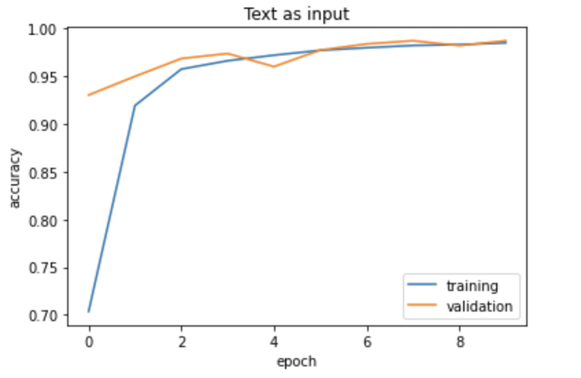
Notice that this model performs slightly better, with a validation accuracy of 98.71% after the 10th epoch. This makes sense, as the text of an article will probably give us more information as to whether or not the article is fake.
Here’s a look at it’s training history.
plot_history(history, title = 'Text')
Now, let’s create a combined model that uses the titles and text of the articles to predict ‘fake news’
First we combine our layers from both previous models:
main = layers.concatenate([title_x, text_x], axis = 1) #combined model
We also create the same final layers as our two previous models. Finally, we create the model, specifying the two inputs (titles and text), and a single output (whether the article is ‘fake’).
main = layers.Dense(32, activation = 'relu')(main) #same last steps as the other models
output = layers.Dense(2, name = 'fake')(main)

#create the model
model3 = keras.Model(
    inputs = [title_input, text_input], #use both inputs
    outputs = output
)
Using the keras.utils.plot_model function, we can also produce a user-friendly visualization of our combined model:
keras.utils.plot_model(model3)
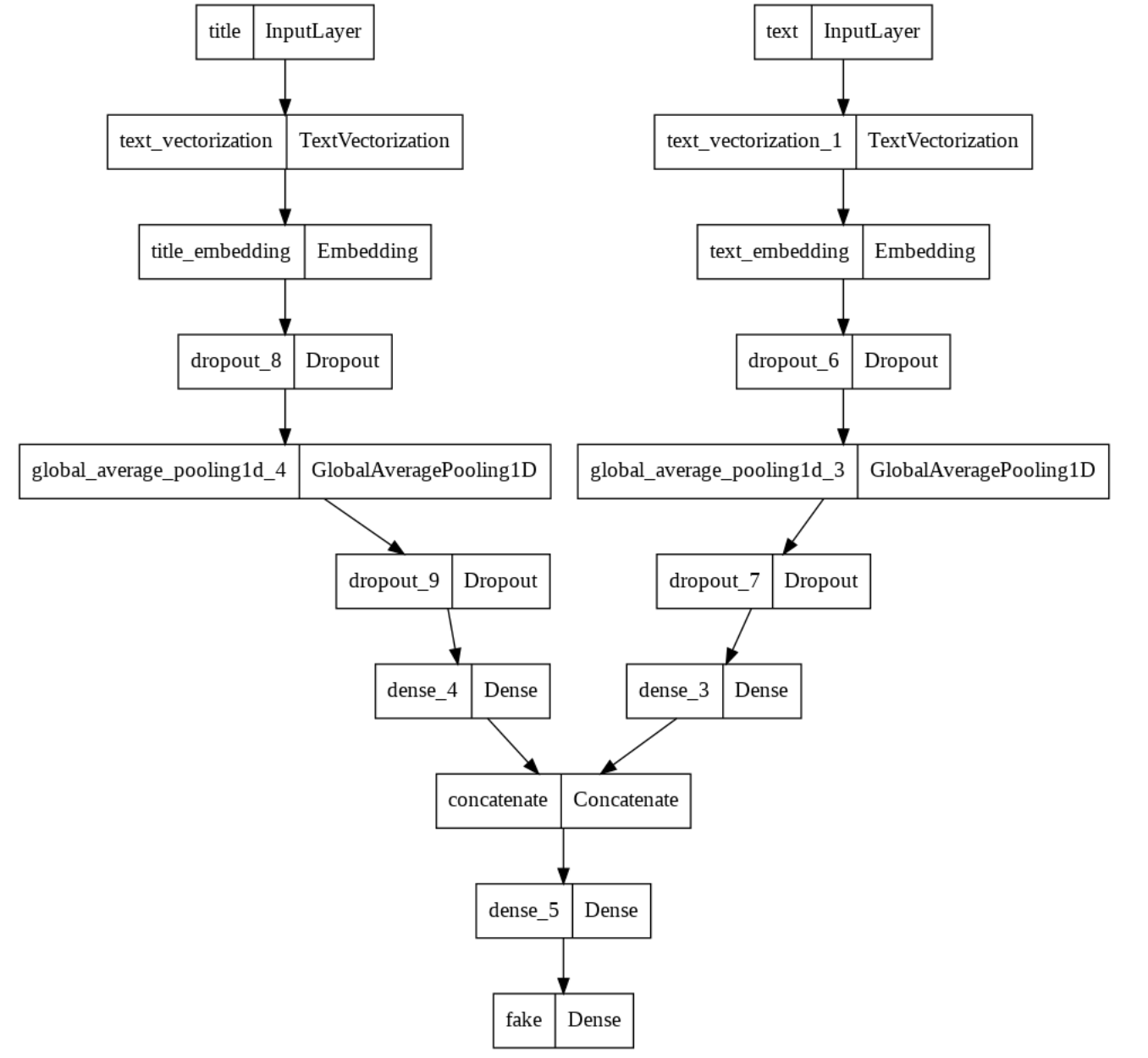 As you can see, the two models function seperately on the titles and text at first, and are then combined into one model. All that’s left is to compile, fit, and train.
model3.compile(optimizer = "adam", #compile the model
              loss = losses.SparseCategoricalCrossentropy(from_logits=True),
              metrics=['accuracy']
)

history = model3.fit(train, #train the model
                    validation_data=val,
                    epochs = 10,
                    verbose = True)
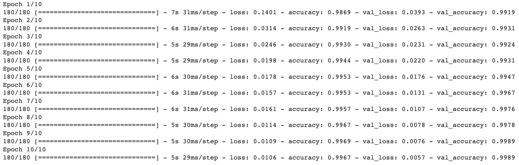 As you can see, this model performs even better than the other two, with a validation accuracy of 99.89%!
Here’s a plot of the training history, notice that the lower bound on the accuracy is around 98.8%.
plot_history(history, title = 'Title and Text')
Step 4: Model Evaluation
Now that we know which model is best, lets evaluate it on the test dataset, which can be found here:
test_url = "https://github.com/PhilChodrow/PIC16b/blob/master/datasets/fake_news_test.csv?raw=true"
We can use our make_dataset function to convert it to the desired format. Then we can evaluate our best model, our combined model3, on the test data,
test_url = "https://github.com/PhilChodrow/PIC16b/blob/master/datasets/fake_news_test.csv?raw=true"
test_df = pd.read_csv(train_url)

test = make_dataset(test_df)

model3.evaluate(test) #evaulate the unseen data
 As we can see, our model performs very well, with an accuracy of 99.77% on the test data!
Step 5: Visualize our Model Embedding
Since our model incorporated a word embedding, we can visualize it to see if we can distinguish any patterns in the words associated with fake or real news.
Notice that above, we used an embedding in 10 dimensions for our titles and text, so to visualize it, we will use PCA to reduce the dimension down to a visualizable number.
Let’s visualize the embedding from our article titles to detect which title words we should look out for when trying to distinguish between real and fake new.
weights = model3.get_layer('title_embedding').get_weights()[0] # get the embedding weights from the embedding layer
vocab = title_vectorize_layer.get_vocabulary() # get the vocabulary from our data prep for later

#apply pca to our embedding weights
from sklearn.decomposition import PCA
pca = PCA(n_components = 2) #'principle component analysis' to reduce dimensions to be able to plot on 2d plane
weights = pca.fit_transform(weights)

#create a dataframe for visualization of the weights along the first two principal components
embedding_df = pd.DataFrame({
    'word' : vocab,
    'x0'   : weights[:,0],
    'x1'   : weights[:,1]
})
embedding_df
 Now, we can visualize these weights using plotly.
import plotly.express as px
from plotly.io import write_html

fig = px.scatter(embedding_df,
                 x = "x0",
                 y = "x1",
                 #size = list(np.ones(len(embedding_df))),
                 size_max = 2,
                 hover_name = "word",
                 title = "Word Embeddings in Article Titles")

fig.show()
write_html(fig, "word_embedding_plotly.html")
 This visualization plots all the words in our data over the first two principal components (x0 and x1). Although here the plot is static, when you run this code in a python environment, the plot is interactive, and thus allows you to distinguish the words by hovering over them. However, we can still make out the words on the extremes.
From this visualization, we see that the words “video”, “breaking”, “wow”,”watch”, “trump’s”, “hillary”, and “obama’s” all appear on the far left, and from the common context in which we see these words in pop culture or news, we can interpret that there is most likely an association between these words and fake news, perhaps used to defame certain politicians.
We also see words like “factbox”,”urges”,”south”, “opposition”,”source” and the names of various countries on the left, which seem to be less commonly used in fake news and more related to actual current events. Thus we could interpret their location as signifying an association with real news.
Interestingly “trump” also appears on the far left, most likely this could be a result of many news articles, fake and real, referring to him, however the distinction that “trump’s” is on the right highlights a key difference between how he might be referenced in fake vs real articles.