
Image Classification with Keras
In this blog post, I’m going to be training various neural networks to perform image classification. More specifically, we will be training these networks to properly classify images of dogs and cats.
First, lets load our data
Here we will read in our data and use the image_dataset_from_directory to load it into TensorFlow objects.
import tensorflow as tf
import os
from tensorflow.keras import utils
from tensorflow.keras import models, layers, losses

# location of data
_URL = 'https://storage.googleapis.com/mledu-datasets/cats_and_dogs_filtered.zip'

# download the data and extract it
path_to_zip = utils.get_file('cats_and_dogs.zip', origin=_URL, extract=True)

# construct paths
PATH = os.path.join(os.path.dirname(path_to_zip), 'cats_and_dogs_filtered')

train_dir = os.path.join(PATH, 'train')
validation_dir = os.path.join(PATH, 'validation')

# parameters for datasets
BATCH_SIZE = 32
IMG_SIZE = (160, 160)

# construct train and validation datasets
train_dataset = utils.image_dataset_from_directory(train_dir,
                                                   shuffle=True,
                                                   batch_size=BATCH_SIZE,
                                                   image_size=IMG_SIZE)

validation_dataset = utils.image_dataset_from_directory(validation_dir,
                                                        shuffle=True,
                                                        batch_size=BATCH_SIZE,
                                                        image_size=IMG_SIZE)

# construct the test dataset by taking every 5th observation out of the validation dataset
val_batches = tf.data.experimental.cardinality(validation_dataset)
test_dataset = validation_dataset.take(val_batches // 5)
validation_dataset = validation_dataset.skip(val_batches // 5)

#snippet to prebatch the data
AUTOTUNE = tf.data.AUTOTUNE

train_dataset = train_dataset.prefetch(buffer_size=AUTOTUNE)
validation_dataset = validation_dataset.prefetch(buffer_size=AUTOTUNE)
test_dataset = test_dataset.prefetch(buffer_size=AUTOTUNE)
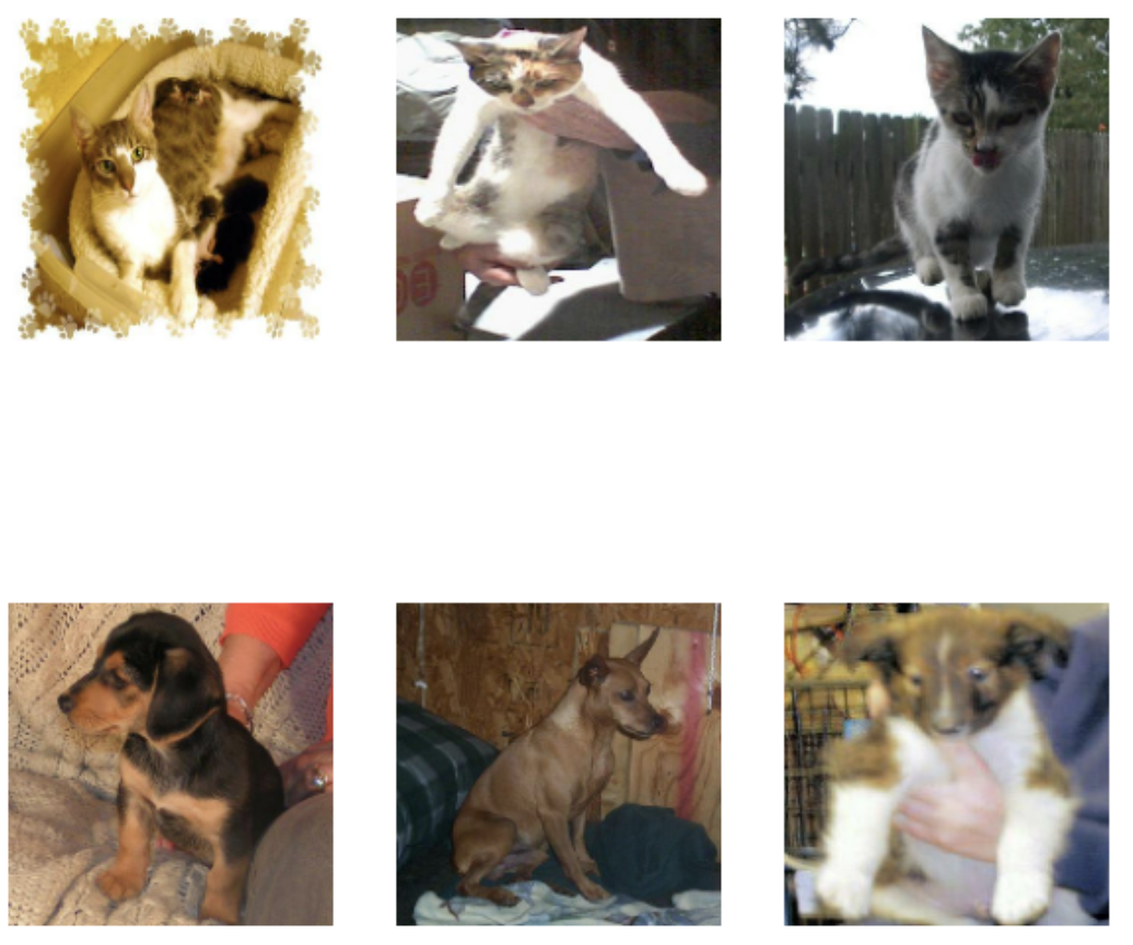
Let’s write a function to visualize our data and see what we’re working with.
import matplotlib.pyplot as plt

def two_row_visualization():
  for image, labels in train_dataset.take(1):
    plt.figure(figsize=(10, 10))
    first_image = image[0]
    cat_images = image[labels == 0]
    dog_images = image[labels == 1]
    for i in range(3):
      ax = plt.subplot(2, 3, i + 1)
      plt.imshow(cat_images[i].numpy().astype("uint8"))
      plt.axis("off")
      ax = plt.subplot(2, 3, i + 4)
      plt.imshow(dog_images[i].numpy().astype("uint8"))
      #lt.title(class_names[labels[i]])
      plt.axis("off")

two_row_visualization()
We can also calculate the number of cats and dogs in our train dataset.
#Check Label Frequencies
labels_iterator= train_dataset.unbatch().map(lambda image, label: label).as_numpy_iterator()
num_cats = 0
num_dogs = 0
for i in labels_iterator:
  if i == 0: num_cats += 1
  if i == 1: num_dogs += 1
print('Number of cats: ',num_cats)
print('Number of dogs: ',num_dogs)
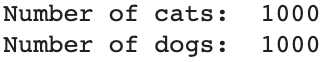 As we can see, there are 1000 of each, thus a baseline classification model would be 50% accurate, as 50% of the images are cats, and 50% of the images are dogs
Next, lets build a model.
First, we will train a CNN model with convolution layers, max_pooling, and a dense layer. Here’s how we do it.
#add layers sequentially

model1 = models.Sequential([
      layers.Conv2D(filters = 32, kernel_size = (3,3), activation = 'relu'),
      layers.MaxPooling2D(pool_size = (2,2)),
      layers.Dropout(0.2),
      layers.Conv2D(filters = 32, kernel_size = (3,3), activation = 'relu'),
      layers.MaxPooling2D(pool_size = (2,2)),
      layers.Dropout(0.2),
      layers.Conv2D(filters = 64, kernel_size = (3,3), activation = 'relu'),
      layers.MaxPooling2D(pool_size = (2,2)),
      layers.Flatten(),
      layers.Dense(64, activation = 'relu'),
      layers.Dense(2)
])

#compile our model
model1.compile(loss=losses.SparseCategoricalCrossentropy(from_logits=True),
optimizer='adam',
metrics=['accuracy'])
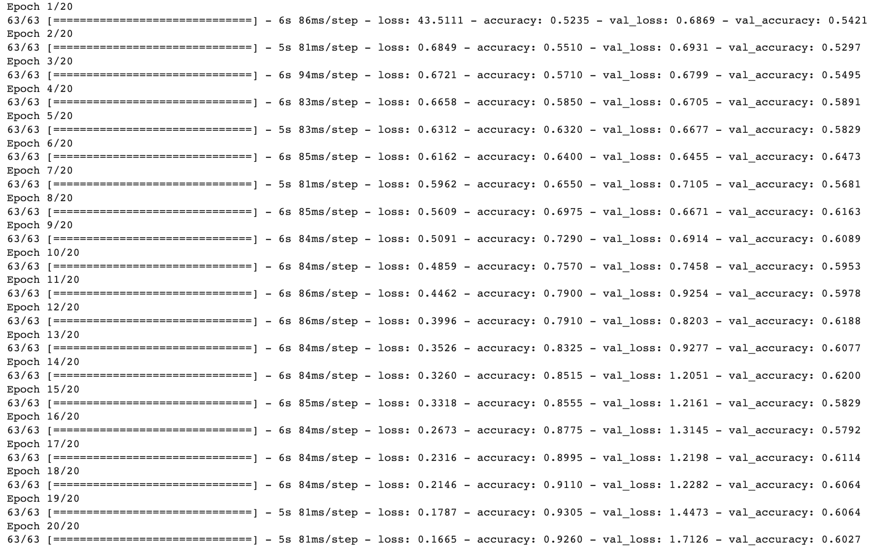
Now that we’ve created the model, we can run it on our training and validation data.
history = model1.fit(train_dataset,
epochs=20,
validation_data=validation_dataset)
Here’s a plot_history function that we can use to plot our training and validation accuracy over time.
def plot_history(history):
plt.plot(history.history["accuracy"], label = "training")
plt.plot(history.history["val_accuracy"], label = "validation")
plt.gca().set(xlabel = "epoch", ylabel = "accuracy")
plt.legend()

plot_history(history)
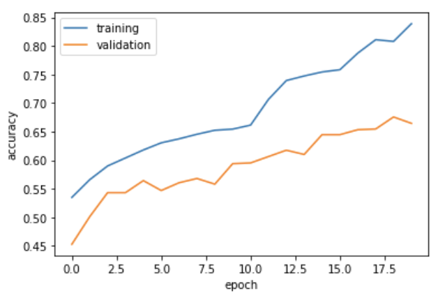
As we can see, our model isn’t incredible, we only achieved an accuracy of about 61% at best.
Let’s try adding some data augmentation to the model
Here we will add a RandomFlip() layer and a RandomRotate() layer to improve the performace of our model. This will flip and rotate the images randomly, allowing the model to learn cat vs. dog classifiction independent from the angle of the image.
First lets implement the Flip and Rotating layers and see what they look like.
flip = layers.RandomFlip(mode = 'vertical')

for images, labels in train_dataset.take(1):
  image = images[0]
plt.figure(figsize=(10, 10))
ax = plt.subplot(1, 4, 1)
plt.imshow(image.numpy().astype("uint8"))
plt.axis("off")
ax = plt.subplot(1, 4, 2)
plt.imshow(flip(image, training = True).numpy().astype("uint8"))
plt.axis("off")
ax = plt.subplot(1, 4, 3)
plt.imshow(flip(image, training = True).numpy().astype("uint8"))
plt.axis("off")
ax = plt.subplot(1, 4, 4)
plt.imshow(flip(image, training = True).numpy().astype("uint8"))
plt.axis("off")
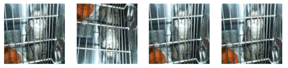
As we can see the images are flipped at random. Next, the random rotation layer:
rotate = layers.RandomRotation(factor = [-1,1])

for images, labels in train_dataset.take(1):
  image = images[0]
plt.figure(figsize=(10, 10))
ax = plt.subplot(1, 4, 1)
plt.imshow(image.numpy().astype("uint8"))
plt.axis("off")
ax = plt.subplot(1, 4, 2)
plt.imshow(rotate(image, training = True).numpy().astype("uint8"))
plt.axis("off")
ax = plt.subplot(1, 4, 3)
plt.imshow(rotate(image, training = True).numpy().astype("uint8"))
plt.axis("off")
ax = plt.subplot(1, 4, 4)
plt.imshow(rotate(image, training = True).numpy().astype("uint8"))
plt.axis("off")

Now that we have these layers, lets add them to our second model.
model2 = models.Sequential([
      layers.RandomFlip(mode = 'vertical', input_shape= (160, 160, 3)),
      layers.RandomRotation(factor = [-1,1]),
      layers.Conv2D(32, (3, 3), activation='relu'),
      layers.MaxPooling2D((2, 2)),
      layers.Dropout(0.2),
      layers.Conv2D(32, (3, 3), activation='relu'),
      layers.MaxPooling2D((2, 2)),
      layers.Dropout(0.2),
      layers.Conv2D(64, (3, 3), activation='relu'), # n "pixels" x n "pixels" x 64
      layers.MaxPooling2D((2, 2)),
      layers.Flatten(), # n^2 * 64 length vector

      layers.Dense(64, activation='relu'),

      layers.Dense(2) # number of classes in your dataset

])

#look at the model
model2.summary()

Let’s train the model.
model2.compile(optimizer='adam',
              loss = tf.keras.losses.SparseCategoricalCrossentropy(from_logits=True),
              metrics = ['accuracy'])


# run model2
history = model2.fit(train_dataset,
                   epochs=20, # how many rounds of training to do
                   #steps_per_epoch = 100, # how many gradient descent steps to do
                   validation_data = validation_dataset)

plot_history(history)
 As we can see, we achieve better accuracy this time, with the best accuracy being about 66%.
Now lets try a third model, in which we add a preprocessing layer.
This layer will normalize and preprocess ou data for improved performance.
i = tf.keras.Input(shape=(160, 160, 3))
x = tf.keras.applications.mobilenet_v2.preprocess_input(i)
preprocessor = tf.keras.Model(inputs = [i], outputs = [x])

model3 = models.Sequential([
      preprocessor,
      layers.RandomFlip(),
      layers.RandomRotation(factor = .2),
      layers.Conv2D(filters = 32, kernel_size = (3,3), activation = 'relu', input_shape = (160,160,3)),
      layers.MaxPooling2D(pool_size = (2,2)),
      layers.Dropout(0.2),
      layers.Conv2D(filters = 32, kernel_size = (3,3), activation = 'relu'),
      layers.MaxPooling2D(pool_size = (2,2)),
      layers.Dropout(0.2),
      layers.Conv2D(filters = 64, kernel_size = (3,3), activation = 'relu'),
      layers.MaxPooling2D(pool_size = (2,2)),
      layers.Flatten(),
      layers.Dense(64, activation = 'relu'),
      layers.Dense(2)
])
#compile model
model3.compile(loss=losses.SparseCategoricalCrossentropy(from_logits=True),
              optimizer='adam',
              metrics=['accuracy'])
              #train model
history = model3.fit(train_dataset,
                     epochs=20,
                     validation_data=validation_dataset)
plot_history(history)
 As we can see, now our model achieves an accuracy of over 70%!
Last model: Transfer Learning
Finally, lets try using a pretrained model. As we will see, this will significantly improve training. First we load the model, then we add it our previous layers.
IMG_SHAPE = IMG_SIZE + (3,)
base_model = tf.keras.applications.MobileNetV2(input_shape=IMG_SHAPE,
include_top=False,
weights='imagenet')
base_model.trainable = False
i = tf.keras.Input(shape=IMG_SHAPE)
x = base_model(i, training = False)
base_model_layer = tf.keras.Model(inputs = [i], outputs = [x])
model4 = models.Sequential([
preprocessor,
layers.RandomFlip(),
layers.RandomRotation(factor = .2),
base_model_layer,
layers.Dropout(0.2),
layers.Flatten(),
layers.Dense(64, activation='relu'),
layers.Dense(2)
])
model4.compile(loss=losses.SparseCategoricalCrossentropy(from_logits=True),
optimizer='adam',
metrics=['accuracy'])
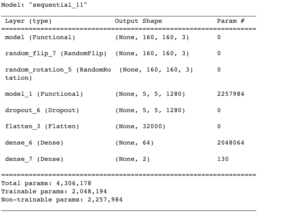
#lets take a look at model4
model4.summary()
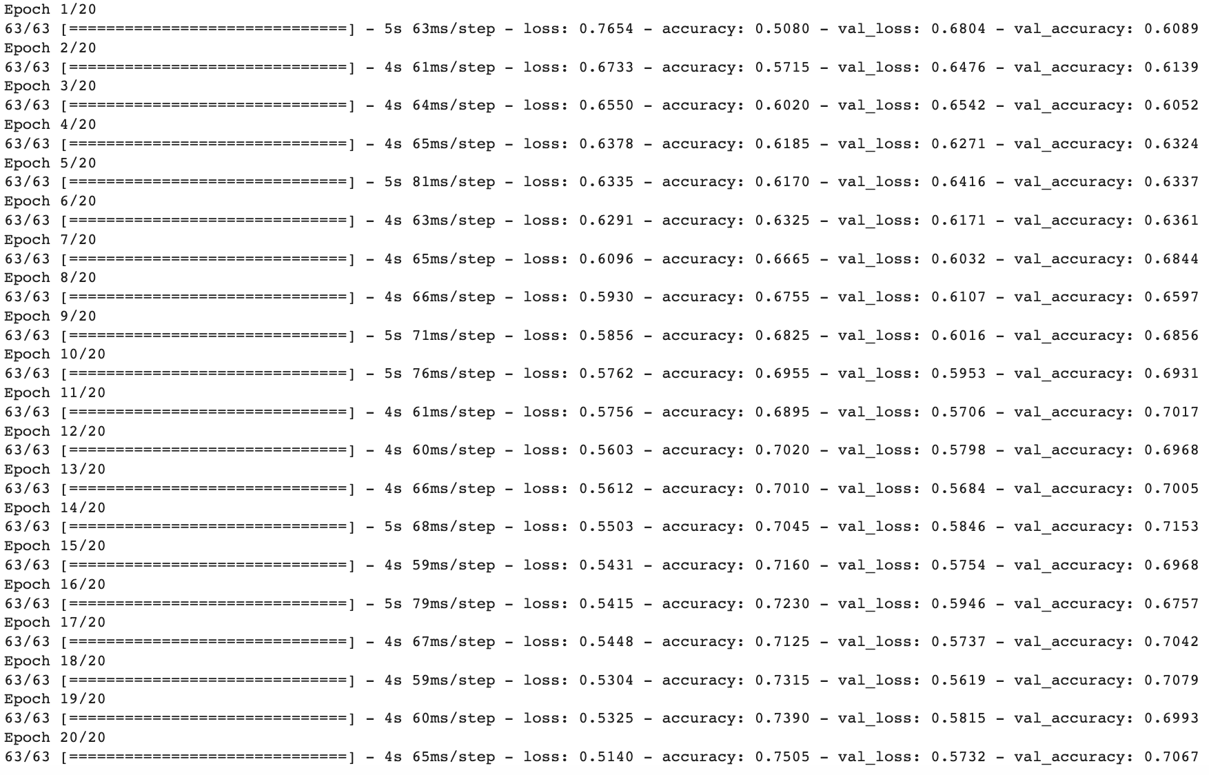
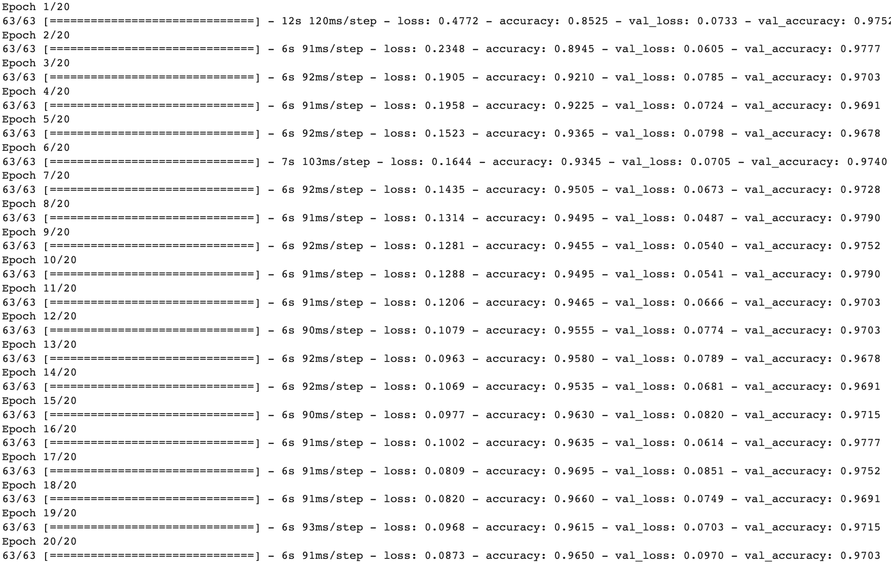
history = model4.fit(train_dataset,
epochs=20,
validation_data=validation_dataset)
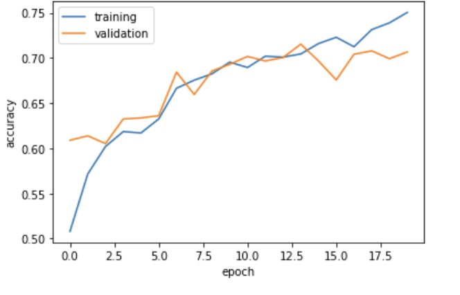
Finally, lets plot its history
plot_history(history)
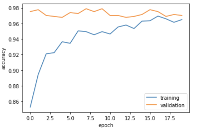
Wow! When training using the pretrained model, we obtain a much higher accuracy, around 97%!
Finally, let’s evaluate our model on the test dataset.
model4.evaluate(test_dataset)

This completes the tutorial, as you can see, adding data augmentation, preprocessing, and using a pretrained model can all contribute toward greatly improving a CNN’s performance!